RF Hacking Intro & Reverse Engineering a Temperature/Humidity Sensor

In this blog post, I will describe how I reverse engineered a few off-the-shelf wireless temperature and humidity sensor after giving an introduction to radio frequency. This has been a really fun journey and I will document the process as thoroughly as I can.
Because there are lots of details, i will try to summarize all the concepts needed to understand how things work.
Introduction
The increasing popularity of Internet of Things (IoT) and other devices becoming wireless is very much apparent in today’s society. With availability of modern Software Defined Radio (SDR) hardware, it has become more accessible, cheaper, and easier than ever to examine the Radio Frequency (RF) signals that are used by these devices to communicate. The following discussion attempts to understand how this communication information is transmitted through RF, and how SDR may be used to analyze and possibly reverse engineer this signal back to understandable data. To achieve this, the RF signals of a number of simple household RF devices will be examined visually in an effort to identify the characteristics of the transmitted signal, along with the data that was transmitted.
Some Basic RF Theory and Terminology
What is Radio Frequency (RF)
To talk about RF, we first have to have some understanding of electromagnetic radiation (EMR). When a charged particle is accelerated through space, such as being emitted by an antenna, it produces two oscillating fields that occur perpendicular to each other, an electric field, and a magnetic field. These oscillating fields are called an EM wave, and can be visualized as shown in the following image, where x is time, E the electric field, and B the magnetic field.

You already know EM waves because we deal with them on a daily basis. Radio waves, microwaves, infrared radiation, visible light, ultraviolet light, x-rays, and gamma-rays, are all EMR. The difference between these types of EMR is the frequency range in which the EM waves oscillate.
RF is generally thought of as EMR with EM wave frequencies in the range of 3kHz to 300GHz, and is mostly used for RADAR and wireless communications. An easy example of RF communication is WiFi, which operates in the 2.4GHz and 5GHz frequency ranges.
For our purposes, we will need to identify a few basic characteristics of EM waves in order to analyze a given signal. These are frequency and wavelength, amplitude, and phase
Frequency and Wavelength
As previously discussed, the frequency of a wave is the rate at which it’s EM fields are oscillating. Generally, the electric field is measured, in which a wave cycle is the oscillating pattern of the wave before that pattern repeats. Frequency (f) is therefore the number of EM wave cycles that occur within a given unit of time. This is generally measured in Hertz (Hz), which is the number of wave cycles per second. This can be seen in the following image, which shows a ten wave cycles of a signal with the frequency of 10 Hz.

Frequency also has a close relationship with the wavelength (λ), which is the distance the wave travels in one wave cycle. As EMR travels at the speed of light through a vacuum, frequency and wavelength are inversely proportional. To calculate this, the formula (λ = f / v) may be used, where v is the velocity in a given medium, generally around 300,000 km/s (approx. speed of light in a vacuum). Frequency is further categorized into frequency bands, which can be seen the following image, also showing the relationship between frequency and wavelength. Why is wavelength important you ask? It directly relates to choosing an appropriate antenna length for a given signal, which we will cover later.
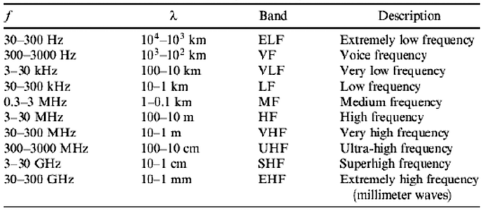
Frequencies are chosen depending on the needs of an application, for instance lower frequencies tend to propagate longer distances than higher frequencies, and is used in applications like over-the-horizon RADAR. Similar frequencies can also interfere with each other, hence why radio stations are separated in frequency. Many countries have government bodies that control the RF spectrum to avoid interference between applications, and regulate RF use. Within Australia, this is the Australian Communications and Media Authority (ACMA). An example of this spectrum allocation can be found here. Only a small portion of the RF spectrum allows transmission without the need for a license.
Amplitude
The amplitude of an RF signal can be thought of as a measure of the change in the electric field oscillation over a a single period. For a sinusoidal wave, this is the magnitude the wave swings above and below a reference value, and can be measured in a few ways, such as peak, peak-to-peak, and root mean square (RMS) amplitude. These are shown in the following image as items 1, 2, and 3, respectively.
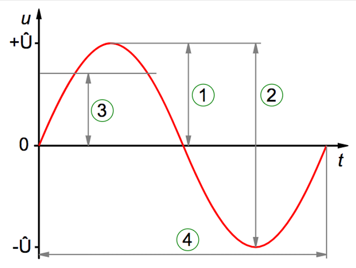
For our purposes, we will only need to observe the changes in amplitude of signals and won’t need to measure this value, however within telecommunications this value is usually a measure of voltage, current, field intensity, or power.
Phase
Lastly let’s have a look at the phase characteristic of an RF signal. The phase of a wave can be thought of as the position of a single point in time during a wave cycle. For a sinusoidal wave this is usually expressed in degrees, or radians, which is shown in the following image.
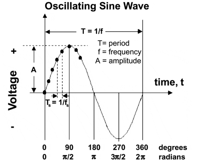
As you can see, if a wave was shifted 180 degrees out of phase, it would be the complete opposite of the original waveform.
Modulation
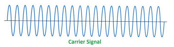
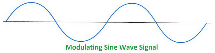
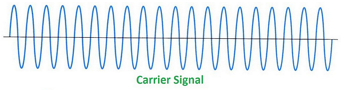
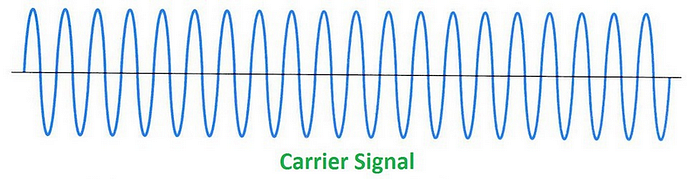
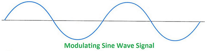
To be useful for any form of communication, an RF signal must have a way to carry information. The previous three wave characteristics, frequency, amplitude, and phase, make up the building blocks for modifying an RF signal in some way to carry data. This is called modulation, and involves mixing a modulating signal, which contains the information to be transmitted, into a periodic waveform called the carrier wave (CW), which propagates the signal through the environment.
Analogue Modulation Schemes
Analogue modulation involves sending an analogue data signal, with an analogue carrier wave. Examples of this would be analogue TV or radio station transmissions. There are a few analogue modulation schemes, however the simplest are amplitude, frequency, and phase modulation.
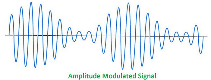
Amplitude Modulation (AM)
With amplitude modulation, the amplitude of the carrier wave is modulated with the data signal. This can be seen in the diagram below
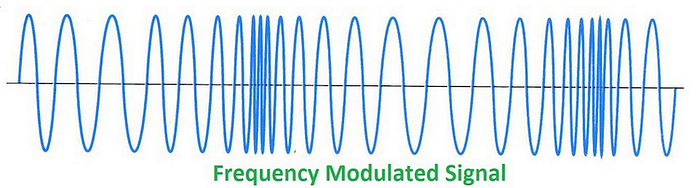
Frequency Modulation (FM)
Frequency modulation can be seen in the diagram below, and shows how the data signal is used to modulate the frequency characteristic of carrier wave.

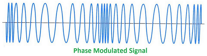
Phase Modulation (PM)
Analogue phase modulation looks very similar to frequency modulation and may be difficult to differentiate the two without some prior knowledge of how the signal is modulated. With this modulation, the carrier wave’s phase is either pushed forward or backward by the modulating data signal.
Digital Modulation
Digital modulation comes from the need to represent a digital signal, i.e. ones and zeros, in the analogue medium of RF for transmission. To achieve this, discrete RF energy states are used to representing some quantity of the digital information, these are called symbols. The three most basic modulation schemes for transmitting digital data are Amplitude Shift Keying, Frequency Shift Keying, and Phase Shift Keying.
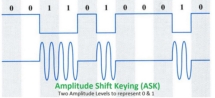
Amplitude Shift Keying (ASK) and On Off Keying (OOK)
ASK involves using the digital data to modulate the amplitude of the carrier wave. This may be by altering the amplitude itself, or simply turning the signal off and on forming a pulse of energy, which is called On-Off Keying (OOK). The following image shows how binary data might modulate the carrier wave through ASK and OOK.
Many forms of RADAR transmit pulses of energy like this, then listen to for the weak reflection of the pulse in order to determine the position of objects in an environment.
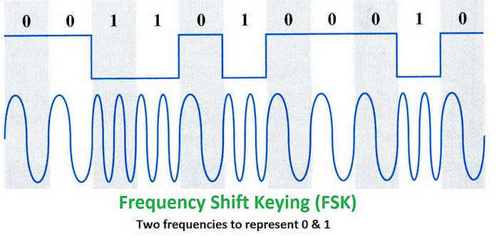
Frequency Shift Keying (FSK)
Similar to ASK, FSK modulates the frequency of the carrier wave with the binary data, forming symbols that have distinct changes in frequency to represent the bits, as seen below.
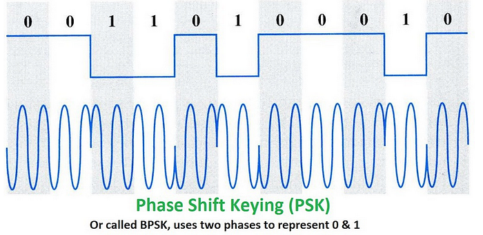
Phase Shift Keying (PSK)
Finally, PSK uses the digital data to modulate the phase of the carrier wave, and forms distinct angular changes in the phase of the signal to represent the binary data as a symbol.
Can You Identify the Modulation in These Captured Signals?
Knowing what we just learned with respect to basic modulation schemes, can you identify the modulation used in the following captured signals? Which are analogue and which are digital?
Note: The animated GIF of each signal shows a waterfall plot of time vs. frequency (higher amplitudes also showing as a brighter green) at the top, with a plot of amplitude vs. frequency at the bottom. The image that follows each animated gif shows a subsection of the waveform which represents the wave’s amplitude vs. time.
Signal 1

Signal 2


Signal 3

Answers:
If you said the first is AM, the second is FM, and the third is ASK or OOK. Then you are correct, however the third signal implements a slightly more complex type of ASK, known as Pulse Duration Modulation (PDM) where the duration of the pulse relates to the modulating data.
Software Defined Radio (SDR)
The example signals above were captured using a hardware SDR device, and displayed using signal analysis software, Baudline.
As radio equipment can be very expensive, and is usually specific to particular applications, SDR solves this problem by removing components that would usually be implemented in hardware, such as mixers, amplifiers, modulators, and demodulators, and implements them in software. This means we can analyze the raw signal being received, however it is up to us to implement the other components in software in order to retrieve the original data. Doing this requires a deeper understanding, but for our purposes we will use inexpensive SDR hardware and software to take a look at some captured signals, and have a go at visually analyzing them.
Hardware Tools
There a several good and relatively inexpensive SDR hardware devices on the market that can be used to receive and transmit RF. The ones used here are the following:
- RTL_SDR
- HackRF One
- YardStick One (not SDR but can be used to receive and transmit modulated signals)
Software Tools
The software tools I found most helpful for capturing and analyzing RF signals on a Linux platform are as follows:
- Baudline (recording and analysis)
- osmocom_fft (recording and analysis)
- Inspectrum (analysis)
- GNU Radio Companion (recording, analysis, demodulation and a whole bunch more)
All these software tools are free, and there are many more out there, including a lot that can automatically demodulate data for specific RF systems.
Note: SDR can be quite resource intensive, the amount of data that is captured in a small time frame can be very large, and also requires high bandwidth from the USB port your SDR device is attached to. This can also cause issues if using virtual machines. There is plenty of information online about setting up SDR devices and software, so Google is your friend here.
Capturing and Analysing RF Signals
Because SDR converts the analogue signal received into digital data, something to note here is the concept of sample rate, and bandwidth. Sample rate refers to the number of samples taken of the analogue signal per second, and directly relates to the bandwidth of the frequency spectrum that is visible at any particular point in time. For example, the higher the sample rate the more frequencies you can see, however this also increases the amount of data being received. The sample rate that is possible depends on your SDR device and the ability of your particular computing resources. Gain is also another important concept, and relates to the amplification of signals. It is worthwhile having a read about these with respect to your particular SDR device.
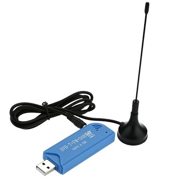
To capture the data, we need an RTL_SDR dongle. But what is it ? RTL stands for Realtek which is a low-cost DVB-T USB dongles.
The RTL-SDR can be used as a wide band radio scanner. Applications include:
- Use as a police radio scanner.
- Listening to EMS/Ambulance/Fire communications.
- Listening to aircraft traffic control conversations.
- Tracking aircraft positions like a radar with ADSB decoding.
- Decoding aircraft ACARS short messages.
- Scanning trunking radio conversations.
- Etc….
Furthermore, with an up-converter or V3 RTL-SDR dongle to receive HF signals the applications are expanded to:
- Listening to amateur radio hams on SSB with LSB/USB modulation.
- Decoding digital amateur radio ham communications such as CW/PSK/RTTY/SSTV.
- Receiving HF weather fax.
- Receiving digital radio mondiale shortwave radio (DRM).
- Listening to international shortwave radio.
- Looking for RADAR signals like over the horizon (OTH) radar, and HAARP signals.
Reconnaissance
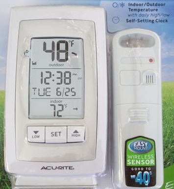
We have a remote temperature sensor at the front door which communicates with the master station over radio, so I decided that reverse engineering the protocol used would be fairly easy task given that I do not have almost any prior SDR experience.
On my Linux, i installed the driver for the rtl_sdr using this tutorial.
After that, i needed to test if it’s working and by then capture some data.
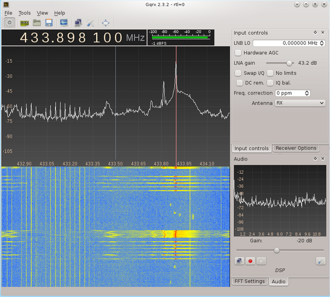
To test, i installed gqrx which is a spectrum analyzer. This last one measures the magnitude of an input signal versus frequency within the full frequency range of the instrument. The primary use is to measure the power of the spectrum of known and unknown signals. Given the challenge of characterizing the behavior of today’s RF devices, it is necessary to understand how frequency, amplitude, and modulation parameters behave over short and long intervals of time.
Tuning the receiver to 433 MHz revealed, that in my area, there is one wide transmission at 433.9 MHz (it seems to persist over the course of a few week, but I have no idea what it is) and a bunch of periodic bursts all over the place. To see, where the station transmits, I disconnected the antenna and brought the dongle closer to the station. It turns out, that the station transmits at 433.6 MHz every ~ 35 seconds. The status LED's blinking correlates with the data being transmitted.
Since it’s a temperature sensor, i needed more than one sample of data, i captured data in 5 different temperature of the day.

As you notice, it stores the frequency, sample rate and the temperature (added by me) in the filename.
To analyze the raw data, i will be using the Universal Hacker Radio (urh).
A good tutorial is provided by Hackin9 to master the basics.
We start by loading the file in the urh to get a general picture of the signal :
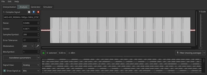
hat doesn’t give us much information about the signal…
First thing I tried is “autodetect parameters” option of urh with different modulations.
ASK:
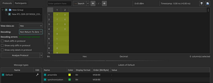
We can consider this as a fail because we can see that it detects that there is only a preamble and a synchronization bytes on the frame. We know that there is a temperature data.
PSK:

The result is different from the previous one: we have a length byte in addition but still no data bytes.
FSK:
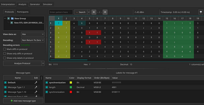
Just similar to the previous one. No data found. I guess we have to manually reverse this protocol…
Manual analysis :
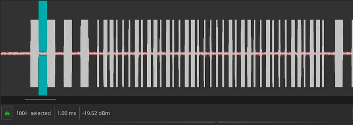
Let’s take a step back and see if we can find something interesting :
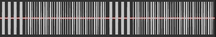
Doesn’t that look like a repeated pattern ?
I loaded the other files and checked if we have the same pattern and it was the case : A pattern is repeated 15 times !
Conclusions:
- There was random looking data followed by a consistent pattern followed by a series of wide and short pulses.
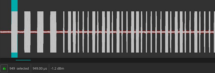
- Eventually I figured out the random pulses at the start of data must be for radio synchronization between the transmitter and receiver.
- None of the “random” data at the start of the bit stream was consistent between any runs and I ended up simply chopping it off and ignoring it in the data stream.
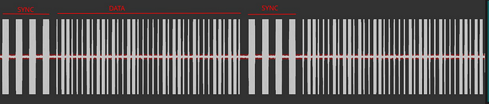
- After the random bits there is a low pulse of varying length followed by 4 data sync pulses.
- The data sync pulses are 0.95 msec.
- Immediately after the 4 data sync pulses are 37 data bit pulses. Each data bit pulse is ~0.72 msec long.
- A logic high (1) bit is encoded as a 0.45 msec high pulse followed by a 0.27 msec low pulse.
- A logic low (0) bit is encoded as a 0.21 msec high followed by a 0.51 msec low.
- The modulation looks like Pulse Width Modulation (PWM)
In URH:
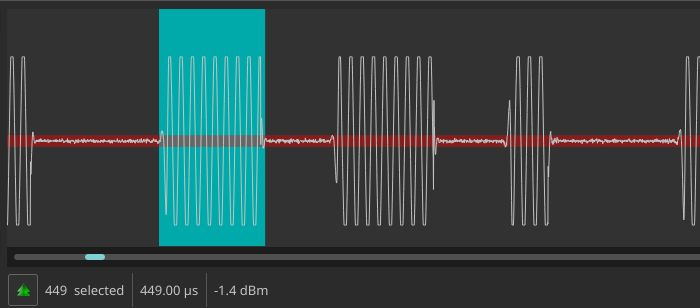
The data synchronization pulses have a duration of 0.95 ms:
Then there is a 1ms of silence :
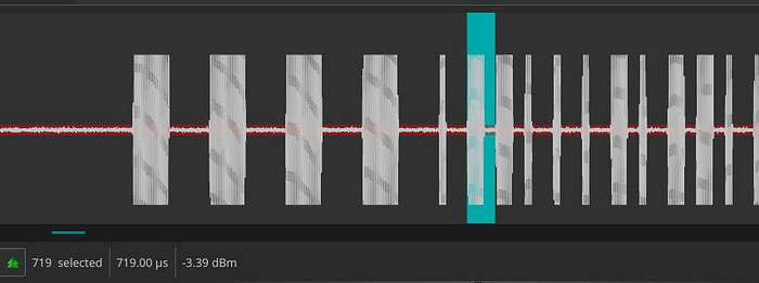
Immediately after the 4 data synchronization pulses, there are 37 data bit pulses :
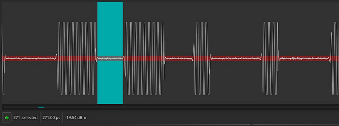
Each data bit pulse lasts approximately 0.72 ms:
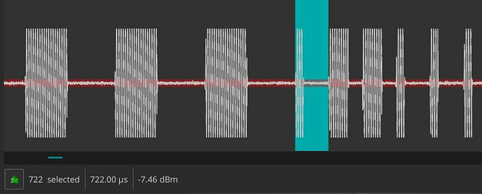
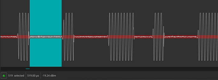
- A logic high (1) bit is encoded as a 0.45 msec high pulse :
followed by a 0.27 msec low pulse :
- A logic low (0) bit is encoded as a 0.21 msec high:

followed by a 0.51 msec low :
Now, it’s time to feed URH a good input so it can decode it for us. Let’s select both type of pulses :
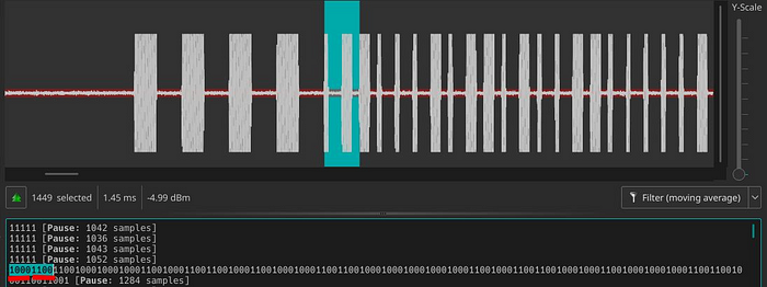
We notice that for the :
- Logic low (0) bit is : 1000
- Logic high (1) bit is : 1100
Each pulse is about 0.72ms, we have 4 bits for each one :
That makes it 0.18ms for a bit.
Let’s add this to URH Sample/Symbol input :
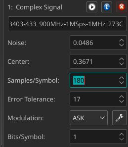
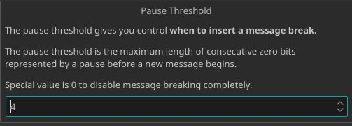
We can also add the value 0000 as silence in the advance parameters :
Last step is to substitute :
- 1100 -> 1
- 1000 -> 0
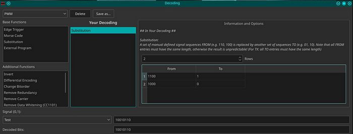
We add our Pulse Width Modulation, then we crop one data frame from 5 samples :
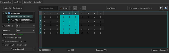
That looks promising ❤
The temperature is surely not represented in the floating representation since it takes more bytes than a normal representation.
I googled how temperature probes encode the data. And i found they do mathematical operations so they remove the float representation and one of the simplest things to do is to multiply it by a power of ten :
For example : 27.3 would be 27.3 * 10¹ = 273
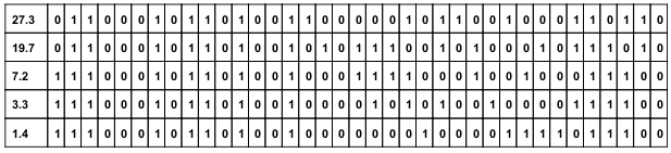
To figure out what has been done in out case, we need to load more files and compare between them :
- 27.3 => 62d30591b
- 19.7 => 62d2b945d
- 7.2 => e2d23c48e
- 3.3 => e2d21521e
- 1.4 => e2d2021ee
We pick the 3 last temperatures because they have the same 3 first bytes.
If we consider the last 2 bytes as a checksum ( it’s the case in a lot of protocol ),
We will be left with :
- 23C
- 215
- 202
The difference between the 1st and 2nd temperature is 0 x27 ( 39 )
And between the 2nd and 3rd is 0 x13 ( 19 ) Exactly as expected because:
72–33 = 39
33–14 = 19
So, they did multiply the temperature by 10 to avoid the floating representation but there is something else : 0x23C is not 77, 0 x215 is not 33,
0x202 is not 14
Quick math:
0x23C = 572
0x215 = 533
0x202 = 514
That’s obvious… They added 500 to each temperature
Let’s verify for the 1st and 2nd temperature :
27.3 * 10 + 500 = 773 = 0x305
19.7 * 10 + 500 = 697 = 0x2b9
Problem solved !
Encoding : Temperature * 10 + 500
Decoding : Temperature — 500 / 10
False data injection
To be able to send temperature, we need to know each field of the packet.
To do that we need to have a binary representation of all the temperatures and compare between them :
After some comparison between the frames and checking temperature sensor’s protocol on the internet (http://wmrx00.sourceforge.net/Arduino/OregonScientific-RF-Protocols.pdf), i reconstructed the most probable frame structure :
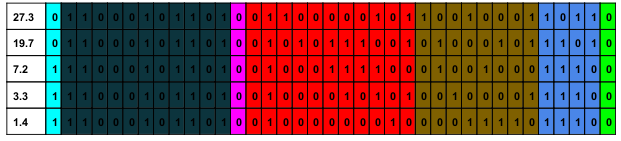
The structure should be :
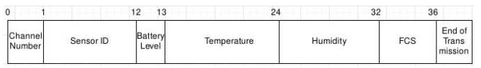
- Channel ID (1bit) : There are 2 channels :
- 0 : for high temperatures
- 1 : for low temperatures - Sensor ID (11bits) : the sensor identifier which is always fixed at 11000101101 (0x62D)
- Battery indicator (1bit) : Indicates the level of the sensor’s battery :
- 0 : High
- 1 : Low - Temperature (11bits): indicates the actual temperature encoded
Humidity (8bits) : indicates the actual humidity percentage in BCD format :
- For 27.3° C: 10010001 (0x91) : 91%
- For 19.7° C: 01000101 (0x43) : 43%
- For 7.2° C: 01001000 (0x48): 48%
- For 3.3° C: 00100001 (0x21): 21%
- For 1.4° C: 00011100 (0x19): 19% - FCS (4bits) : Frame checksum, calculated using this formula :
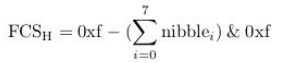
- End Of Transmission (1bit) : a fixed bit to the value of 0, indicates the end of transmission
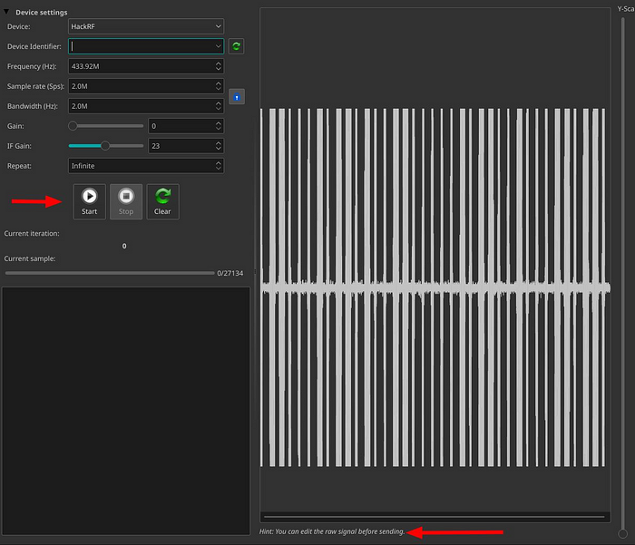
Now, to send any false data to the weather station, we can just edit a frame, recalculate the FCS and play it in URH :
What Have We Learned?
We looked at some RF theory to get a good basic understanding of what RF is, how data is transmitted using RF signals, and discussed some common analogue and digital modulation schemes that are the basis of more complex modulation. We briefly described SDR, including some hardware and software SDR tools that are useful for RF signal analysis and reverse engineering, along with tips for using those tools to capture and view RF signals. We identified a good methodology for attempting to reverse engineer and understand wireless protocols, and finally, we looked at the RF signals produced by some common devices in an effort to determine their characteristics, and identified some security issues along the way.
Although this discussion is not exactly a deep guide on reversing RF signals with SDR, hopefully you have learned something, or at least found it an interesting read.
Please, if you notice that i miss understood something, let me know ^_^
Stay tuned for a 2nd part of RF Hacking =D
#Yan1x0s
